Right Censoring with survivalMPL

Overview

A survival time is right censored when follow-up ends before the event occurs: all we know is that the event time exceeds the last observation time. This is the most common censoring scheme, and the one survival::coxph() handles through the partial likelihood.

coxph_mpl() fits the same proportional hazards model, but estimates the baseline hazard $h_0$ jointly with $\boldsymbol{\beta}$ instead of profiling it out. The practical consequence is that a fit gives absolute hazard and survival estimates directly, with standard errors, rather than requiring a separate Breslow-type step afterwards.

Encoding right-censored observations

Right-censored data use the ordinary two-argument response, exactly as in coxph():

Surv(time, status)

where status is 1/TRUE for an observed event and 0/FALSE for a censored observation. This is the one scheme that does not need type = "interval2"; internally coxph_mpl() converts it to that form anyway.

Example: `survival::lung`

The lung data from the survival package records survival in patients with advanced lung cancer. status is coded 2 for death and 1 for censored, so the event indicator is status == 2.

library(survivalMPL)
#> Loading required package: survival
#> Loading required package: MASS
library(survival)

lung <- na.omit(lung[, c("time", "status", "age", "sex", "ph.karno", "wt.loss")])

c(n = nrow(lung), events = sum(lung$status == 2),
  censored = sum(lung$status == 1))
#>        n   events censored 
#>      214      152       62

Model fit

Little beyond the formula and the data is required. The defaults use a uniform (piecewise-constant) baseline hazard, take the number of knots from the number of events, and select the smoothing value $\lambda$ automatically by the marginal likelihood method. The one change made here is the convergence tolerance, set to the $10^{-5}$ used throughout Ma et al. (2024); at the default $10^{-7}$ the outer iterations do not settle on this dataset - see Control Parameters:

fit_lung <- coxph_mpl(
  Surv(time, status == 2) ~ age + sex + ph.karno + wt.loss,
  data = lung,
  tol  = 1e-05
)

summary(fit_lung)
#> 
#> coxph_mpl(formula = Surv(time, status == 2) ~ age + sex + ph.karno + 
#>     wt.loss, data = lung, tol = 1e-05)
#> 
#> -----
#> 
#> Cox Proportional Hazards Model Fit Using MPL 
#> 
#> 
#> Penalized log-likelihood  :  -1059.173
#> Estimated smoothing value :  5945063
#> Convergence               :  Yes (101 + 571 iter.) 
#> 
#> Data             : lung
#> Number of obs.   : 214
#> Number of events : 152 (71.02804%)
#> Number of cens.  :  62 (28.97196%)
#> 
#> Regression parameters : Surv(time, status == 2) ~ age + sex + ph.karno + wt.loss
#>            Estimate Std. Error z-value Pr(>|z|)   
#> age       0.0144154  0.0101531  1.4198 0.155666   
#> sex      -0.5103399  0.1708342 -2.9873 0.002814 **
#> ph.karno -0.0117159  0.0089906 -1.3031 0.192529   
#> wt.loss  -0.0017065  0.0071640 -0.2382 0.811722   
#> ---
#> Signif. codes:  0 '***' 0.001 '**' 0.01 '*' 0.05 '.' 0.1 ' ' 1
#> 
#> Baseline hasard parameters approximated using Uniform :
#>  (11 equal events bins)
#>           1           2           3           4           5           6 
#> 0.003163491 0.003488916 0.004576128 0.005400816 0.005924636 0.006389894 
#>           7           8           9          10          11 
#> 0.006875642 0.007437590 0.007988655 0.008295504 0.008327673 
#> 
#> -----

The coefficient table is read as in any Cox fit: sex is strongly protective (coded 1 = male, 2 = female), and higher ph.karno (better performance status) is associated with lower hazard. The summary also reports the estimated baseline hazard coefficients $\boldsymbol{\theta}$ , which have no counterpart in a partial likelihood fit.

Every one of those defaults can be overridden through coxph_mpl.control() - the basis, the knots, the smoothing parameter, the iteration limits. The Control Parameters article covers them one at a time.

Baseline hazard and survival

Because $h_0$ is part of the model, it can be plotted with confidence bands straight from the fitted object. plot() produces four panels: the basis functions, then the estimated baseline hazard, cumulative hazard and survival.

par(mfrow = c(2, 2), mar = c(4, 4, 3, 1))
plot(fit_lung, ask = FALSE, cex.main = 0.8)

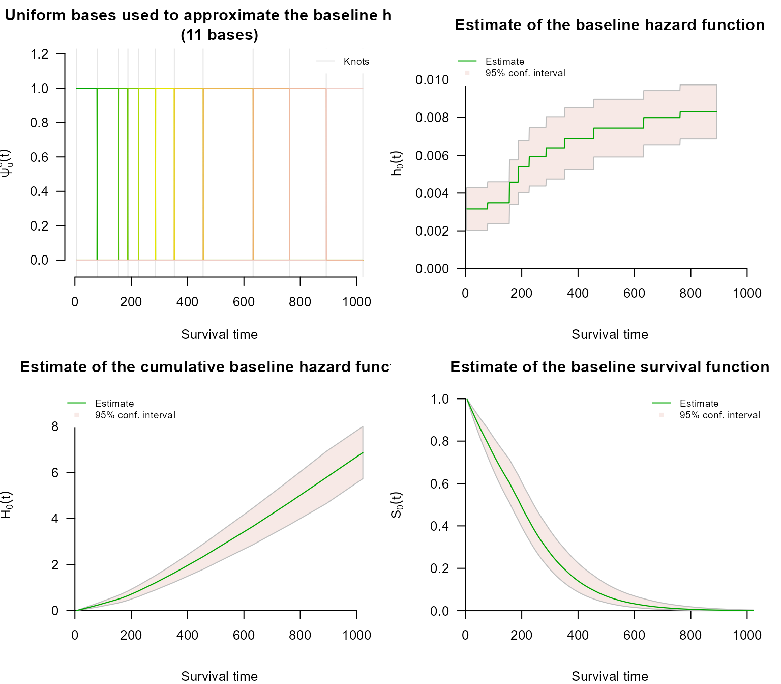
In the first panel each of the $m$ basis functions is drawn in its own colour, running through terrain.colors() from the earliest to the latest, so the colour simply indexes $u$ in $\psi_u$ and carries no other meaning. With the default uniform basis each $\psi_u$ is an indicator on one knot interval, so the panel reads as a row of adjacent boxes of height 1, one colour per interval; the pale grey verticals are the knots $\boldsymbol{\alpha}$ . A basis drawn dashed would indicate $\hat\theta_u$ driven to zero, meaning that interval contributes nothing to the fitted hazard.

The second panel is the estimated baseline hazard itself: a step function whose height on knot interval $u$ is $\hat\theta_u$ . It is the one quantity a partial likelihood fit cannot give you, so it is worth drawing on its own:

plot(fit_lung, which = 2, ask = FALSE, cex.main = 0.9)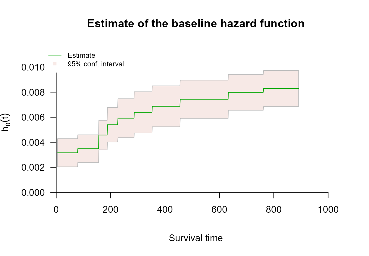

The hazard climbs steadily across follow-up - more than doubling between the first knot interval and the last - and flattens only in the final intervals, where few patients remain at risk and the confidence band widens accordingly.

Predicted survival

predict() returns absolute estimates with standard errors and pointwise confidence limits. With no i argument it evaluates at the mean covariate vector:

pred_lung <- predict(fit_lung, type = "survival")
head(pred_lung)
#>        time  survival           se       low      high
#> 1  4.999000 1.0000000 0.0000000000 1.0000000 1.0000000
#> 2  6.017019 0.9985435 0.0002149955 0.9981135 0.9989734
#> 3  7.035038 0.9970890 0.0004293647 0.9962303 0.9979478
#> 4  8.053057 0.9956367 0.0006431090 0.9943505 0.9969229
#> 5  9.071076 0.9941865 0.0008562298 0.9924741 0.9958990
#> 6 10.089095 0.9927385 0.0010687283 0.9906010 0.9948759

A single subject is selected with i (one row index at a time; only the first element is used):

pred_one <- predict(fit_lung, type = "survival", i = 1)
head(pred_one)
#>        time  survival           se       low      high
#> 1  4.999000 1.0000000 0.0000000000 1.0000000 1.0000000
#> 2  6.017019 0.9982519 0.0002579962 0.9977359 0.9987679
#> 3  7.035038 0.9965068 0.0005150903 0.9954766 0.9975370
#> 4  8.053057 0.9947648 0.0007712848 0.9932222 0.9963074
#> 5  9.071076 0.9930258 0.0010265820 0.9909727 0.9950790
#> 6 10.089095 0.9912899 0.0012809843 0.9887279 0.9938519

Residuals

residuals() returns both Cox-Snell and martingale residuals. For a subject observed exactly, the Cox-Snell residual is the fitted cumulative hazard that subject accumulated,

$r^{CS}_i = e^{\mathbf{x}_i^T\hat{\boldsymbol{\beta}}}\,\hat H_0(t_i),$

with censored observations adjusted so that every residual estimates the same quantity under the model. The martingale residual is then $\hat M_i = \delta_i - r^{CS}_i$ : the difference between the number of events actually observed for subject $i$ (0 or 1) and the number the model expects.

res_lung <- residuals(fit_lung)
par(mfrow = c(1, 2), mar = c(4, 4, 3, 1))
plot(res_lung, which = 1:2, ask = FALSE)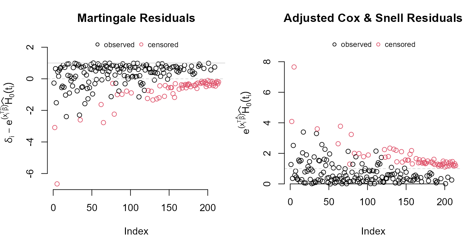

Read them as follows.

Martingale residuals are bounded above by 1 and unbounded below, so the cloud is asymmetric by construction: censored observations (red) are at or below zero, events (black) are pulled towards 1. A residual close to 1 marks a subject who died far earlier than the model predicted, a large negative one a subject who survived far longer. Here a handful of subjects sit below $-2$ , one of them near $-6$ : those are the long survivors the fitted model finds most surprising, and they are worth looking at individually before concluding anything about the model as a whole.
Cox-Snell residuals behave like a censored sample from a unit exponential distribution when the model is correct, so most sit below 1 with a thinning right tail. A mass of residuals far above 1 indicates the fitted cumulative hazard is wrong, usually through a mis-specified covariate effect rather than a mis-specified baseline.

The horizontal axis of both panels is the row number, which carries meaning only if the rows arrived in a meaningless order. In lung they did not: the censored subjects are concentrated in the later rows (3 of the first 54 are censored, against 36 of the last 53), which is why the red points drift to the right of both panels. That is a fact about the data file, not about the fit.

Next steps

Control Parameters covers coxph_mpl.control(): the basis, the knots, the smoothing value $\lambda$ , the iteration limits and the convergence tolerance used above.
Left Truncation covers delayed entry, where subjects join the risk set only at some entry time. Right-censored data are often also left truncated, and coxph_mpl() handles it through the entry argument.
Interval Censoring covers the other censoring scheme, which uses the type = "interval2" response.
Basis Functions for the Baseline Hazard explains the four choices for $\psi_u$ and how the knots are placed.
Comparing coxph() and coxph_mpl() fits both to the same right-censored data and contrasts the results.

References

Ma, Jun, Annabel Webb, and Harold Malcolm Hudson. 2024. Likelihood Methods in Survival Analysis: With R Examples. 1st ed. Chapman; Hall/CRC. https://doi.org/10.1201/9781351109710.