Left Truncation with survivalMPL • survivalMPL

Overview

A survival time is left truncated when any event occurring before some time $a_i$ could never have been observed at all. The truncation time is also called a delayed entry time, because it usually arises from a condition on entering the study: a subject who fails before meeting that condition never appears in the data.

Truncation is not censoring, and the difference is fundamental. Censoring means a survival time is only partially observed: the subject is in the data, and contributes the information that the event had not yet happened. Truncation means an event time that could have been observed becomes entirely unobservable when it falls before $a_i$ : the subject is absent from the data altogether. Treating a truncation time as time zero for follow-up, and so ignoring the truncation, leads to biased parameter estimates (Bhaskaran et al., n.d.).

Each subject therefore contributes $(a_i, y_i, \delta_i, \mathbf{x}_i)$ : the truncation time, the observed event or censoring time, the event indicator, and the covariates, with $a_i$ strictly less than $y_i$ .

Encoding left-truncated observations

Truncation times are not part of the Surv() response. Pass them through the entry argument instead:

coxph_mpl(Surv(time, status) ~ x, data = df, entry = start)

Three things to know:

entry requires basis = "uniform", which is the default, so nothing else has to be set. Left truncation is implemented by differencing the cumulative basis, $H_0(a_i, y_i) = H_0(y_i) - H_0(a_i)$ , which the package supports for the piecewise-constant basis. This is not a limitation of the method so much as its natural setting: with indicator basis functions $\psi_u(t) = I(t \in B_u)$ over bins $B_u = (w_u, w_{u+1}]$ , each $\hat\theta_u$ has a closed form given $\boldsymbol{\beta}$ , which is what makes the profile likelihood of Bhaskaran et al. (n.d.) possible. Asking for any other basis together with entry gets you a uniform fit and a warning saying so, rather than a silently wrong fit or a refusal.
Entry times must strictly precede the event or censoring time. A violation is an error, not a warning.
Truncated and untruncated subjects may be mixed in one call. Use an entry time of zero, or any value below the first event time, for subjects observed from the origin.

Example: atomic bomb survivors

The bundled hiroshima data are left truncated by construction. Follow-up in the Life Span Study begins on 1 October 1950, several years after the 1945 exposure, so a subject enters the risk set at the age they had reached by that date, and anyone who died in between is absent from the cohort. entry is that attained age, and time is attained age at death or at end of follow-up.

library(survivalMPL)
#> Loading required package: survival
#> Loading required package: MASS
library(survival)

data(hiroshima)

c(subjects = nrow(hiroshima), deaths = sum(hiroshima$status))
#> subjects   deaths 
#>    86611    50620
round(range(hiroshima$entry), 1)
#> [1]  5.2 93.8
round(range(hiroshima$time), 1)
#> [1]   7.0 114.9

Entry ages run from 5 to 94 years, so the truncation is substantial rather than incidental: at any attained age, the subjects at risk are only those who had already reached that age by late 1950.

fit_entry <- coxph_mpl(
  Surv(time, status) ~ dose + sex + city,
  data  = hiroshima,
  entry = entry
)

summary(fit_entry)
#> 
#> coxph_mpl(formula = Surv(time, status) ~ dose + sex + city, data = hiroshima, 
#>     entry = entry)
#> 
#> -----
#> 
#> Cox Proportional Hazards Model Fit Using MPL 
#> 
#> 
#> Penalized log-likelihood  :  -218085.3
#> Estimated smoothing value :  486.6378
#> Convergence               :  Yes (12 + 292 iter.) 
#> 
#> Data             : hiroshima
#> Number of obs.   : 86611
#> Number of events : 50620 (58.44523%)
#> Number of cens.  : 35991 (41.55477%)
#> 
#> Regression parameters : Surv(time, status) ~ dose + sex + city
#>                Estimate Std. Error  z-value  Pr(>|z|)    
#> dose          0.1635084  0.0151308  10.8063 < 2.2e-16 ***
#> sexFemale    -0.5518858  0.0092909 -59.4005 < 2.2e-16 ***
#> cityNagasaki  0.0515481  0.0098435   5.2368 1.634e-07 ***
#> ---
#> Signif. codes:  0 '***' 0.001 '**' 0.01 '*' 0.05 '.' 0.1 ' ' 1
#> 
#> Baseline hasard parameters approximated using Uniform :
#>  (11 equal events bins)
#>           1           2           3           4           5           6 
#> 0.001058039 0.002478473 0.004673498 0.009799451 0.019100936 0.033959813 
#>           7           8           9          10          11 
#> 0.062309691 0.111161804 0.214221247 0.340579097 0.348117394 
#> 
#> -----

The estimated baseline hazard is a hazard by attained age, and because the risk set at each age contains only subjects who had already reached that age by late 1950, it is the truncation-corrected one:

plot(fit_entry, which = 2, ask = FALSE, cex.main = 0.9)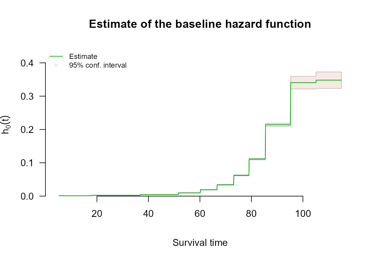

Requesting a different basis alongside entry does not fail; the fit falls back to "uniform" and says so:

fallback <- coxph_mpl(
  Surv(time, status) ~ dose + sex + city,
  data  = hiroshima,
  entry = entry,
  basis = "msplines"
)
#> Warning: entry= (left truncation) is only implemented for basis = "uniform";
#> basis "msplines" was replaced by "uniform".

fallback$control$basis
#> [1] "uniform"

Limitations

predict.coxph_mpl() and residuals.coxph_mpl() do not yet account for entry: they compute cumulative hazard and survival from time zero rather than from each subject’s entry time. Coefficients, baseline hazard estimates and their standard errors are unaffected. See ?coxph_mpl for the current status.

References

Bhaskaran, Aishwarya, Benoit Liquet, and Jun Ma. n.d. Maximum Profile Likelihood for Cox Models Under Left Truncation and Right Censoring. Macquarie University.