Basis Functions for the Baseline Hazard

The MPL baseline hazard expansion

The Cox proportional hazards model specifies the hazard for subject $i$ as

$h(t_i) = h_0(t_i)\,e^{\mathbf{x}_i^T \boldsymbol{\beta}},$

where $\boldsymbol{\beta}$ collects the regression coefficients and $h_0(\cdot)$ is an unspecified baseline hazard. Maximum penalised likelihood (MPL) estimation approximates $h_0$ by a finite mixture of non-negative basis functions $\psi_1, \ldots, \psi_m$ :

$h_0(t) = \sum_{u=1}^{m} \theta_u\,\psi_u(t), \qquad H_0(t) = \int_{t_{(1)}}^{t} h_0(v)\,dv = \sum_{u=1}^{m} \theta_u\,\Psi_u(t),$

where $\Psi_u(t) = \int_{t_{(1)}}^{t}\psi_u(v)\,dv$ is the cumulative basis and $\boldsymbol{\theta} = (\theta_1,\ldots,\theta_m)^T \geq \mathbf{0}$ are coefficients estimated alongside $\boldsymbol{\beta}$ (Ma et al. 2014, 2024).

survivalMPL provides four production basis types, selectable via the basis argument of coxph_mpl.control():

`basis` string	Description
`"uniform"` (or `"u"`)	Piecewise-constant (step function)
`"gaussian"` (or `"g"`)	Truncated Gaussian kernels
`"msplines"` (or `"m"`)	M-splines of order $o$
`"epanechikov"` (or `"e"`, `"epanechnikov"`)	Epanechnikov kernels

The rest of this article presents the mathematical definition of each basis, visualises the shapes, and compares fits on the bundled melanoma dataset.

Uniform (step-function) basis

The time range $[t_{(1)}, t_{(n)}]$ is partitioned into $m$ adjacent intervals $[\alpha_u, \alpha_{u+1})$ . The density and cumulative bases are

$\psi_u(t) = \mathbf{1}(\alpha_u \leq t < \alpha_{u+1}),$

$\Psi_u(t) = \mathbf{1}(\alpha_u \leq t) \Bigl[t^{\mathbf{1}(t < \alpha_{u+1})}\,\alpha_{u+1}^{\mathbf{1}(\alpha_{u+1} \leq t)} - \alpha_u\Bigr].$

Each $\theta_u$ is then interpreted directly as the constant hazard rate on $[\alpha_u, \alpha_{u+1})$ .

Gaussian basis

Basis function $u$ is a truncated Gaussian density centred at knot $\alpha_u$ with scale $\sigma_u$ :

$\psi_u(t) = \frac{1}{\sigma_u\,\delta_u}\, \phi\!\left(\frac{t - \alpha_u}{\sigma_u}\right), \qquad \Psi_u(t) = \frac{1}{\delta_u} \left[\Phi\!\left(\frac{t - \alpha_u}{\sigma_u}\right) -\Phi\!\left(\frac{t_{(1)} - \alpha_u}{\sigma_u}\right)\right],$

where $\phi$ and $\Phi$ are the standard normal density and CDF, and $\delta_u = \Phi\!\left(\tfrac{t_{(n)}-\alpha_u}{\sigma_u}\right) -\Phi\!\left(\tfrac{t_{(1)}-\alpha_u}{\sigma_u}\right)$ ensures each truncated basis integrates to 1 on $[t_{(1)}, t_{(n)}]$ .

M-spline basis

M-splines of order $o$ are built recursively from augmented knots $\boldsymbol{\alpha}^\star = \bigl[\alpha_1 \mathbf{1}_{o-1}^T,\,\boldsymbol{\alpha}^T,\,\alpha_{n_\alpha}\mathbf{1}_{o-1}^T\bigr]^T$ :

$\psi^o_u(t) = \begin{cases} \dfrac{\mathbf{1}(\alpha^\star_u \leq t < \alpha^\star_{u+1})} {\alpha^\star_{u+1} - \alpha^\star_u} & o = 1,\\[8pt] \dfrac{o}{o-1} \dfrac{\mathbf{1}(\alpha^\star_u \leq t < \alpha^\star_{u+o})} {\alpha^\star_{u+o} - \alpha^\star_u} \Bigl[(t-\alpha^\star_u)\,\psi^{o-1}_u(t) +(\alpha^\star_{u+o}-t)\,\psi^{o-1}_{u+1}(t)\Bigr] & \text{otherwise.} \end{cases}$

The cumulative $\Psi^o_u(t)$ is an I-spline (integrated M-spline); each $\psi^o_u$ integrates to 1 over its support $[\alpha^\star_u, \alpha^\star_{u+o}]$ . survivalMPL defaults to $o = 3$ (cubic M-splines), for which the second-order roughness penalty has a closed form.

Epanechnikov basis

Epanechnikov basis functions have compact parabolic support. For the interior functions ( $1 < u < m$ ):

$\psi_u(t) = \frac{6\,\mathbf{1}(\alpha^\star_u \leq t < \alpha^\star_{u+o}) (t - \alpha^\star_u)(t - \alpha^\star_{u+o})}{(\alpha^\star_u - \alpha^\star_{u+o})^3}.$

The endpoint functions ( $u = 1$ and $u = m$ ) use asymmetric variants to ensure a proper probability density on their support. Like M-splines, these use the augmented knot sequence $\boldsymbol{\alpha}^\star$ .

Visual comparison

The code below uses the package’s internal basis machinery to evaluate $\psi_u(t)$ on a fine grid and plot each set of basis functions.

n.knots = c(k_1, k_2) places $k_1 + 1$ quantile-based knots over the lower range.quant[2] (90% by default) of the event times, plus $k_2 + 1$ equally spaced knots above that quantile, giving $k_1 + k_2 + 2$ knots in total. The defaults are c(8, 2) for "uniform" and "msplines" (12 knots, $m = 11$ and $13$ ) and c(0, 20) for "gaussian" and "epanechikov" (22 knots, $m = 22$ and $23$ ).

The figure below deliberately uses far fewer: n.knots = c(0, 6), i.e. 8 widely spaced knots and $m = 7$ to $9$ basis functions per panel. At the default resolution the curves overlap into a dense, unreadable thicket, and on this right-skewed dataset the quantile knots crowd so tightly near $t = 0$ that the first basis function spikes and flattens all the others. Fewer knots do not change the shape of an individual basis function, only how many there are and how wide each one is.

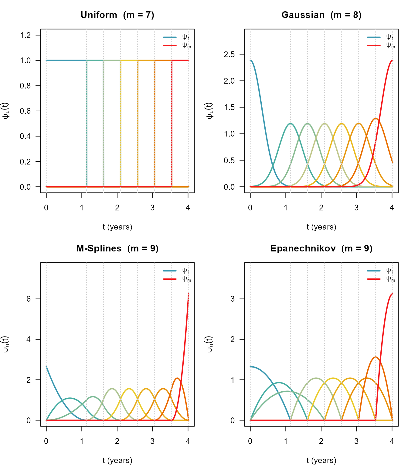
Colour runs with the basis index: $\psi_1$ (blue) is left-most in time, $\psi_m$ (red) right-most. Dotted vertical lines mark the knots $\boldsymbol{\alpha}$ .

Fitting comparison on `melanoma`

The choice of basis affects the smoothness and shape of the estimated baseline hazard but rarely changes regression coefficient estimates substantially. Here we fit the same interval-censored model with all four bases using the bundled pseudo-melanoma data (time to first local recurrence, $n = 300$ , true baseline $h_0(t) = t^{-1/2}$ ).

All four fits share the same knot specification, n.knots = c(8, 2), so that the comparison is between basis shapes and not between different numbers of parameters. (The defaults differ by basis: "uniform" and "msplines" use c(8, 2), while "gaussian" and "epanechikov" use c(0, 20).)

data(melanoma)
formula_mel <- Surv(t_L, t_R, type = "interval2") ~
  Arm + Leg + Trunk + mm1to2 + mm2to4 + mm4plus + Female + Age_centred
n_obs <- sum(melanoma$t_L == melanoma$t_R & is.finite(melanoma$t_R))
base_ctrl <- list(n.obs = n_obs,
                  smooth = 0,
                  n.knots = c(8, 2),
                  max.iter = c(40, 2e4, 5e4))

fit_u <- coxph_mpl(formula_mel, data = melanoma,
  control = do.call(coxph_mpl.control,
    c(base_ctrl, list(basis = "uniform"))))

fit_g <- coxph_mpl(formula_mel, data = melanoma,
  control = do.call(coxph_mpl.control,
    c(base_ctrl, list(basis = "gaussian"))))

fit_m <- coxph_mpl(formula_mel, data = melanoma,
  control = do.call(coxph_mpl.control,
    c(base_ctrl, list(basis = "msplines"))))

fit_e <- coxph_mpl(formula_mel, data = melanoma,
  control = do.call(coxph_mpl.control,
    c(base_ctrl, list(basis = "epanechikov"))))

Regression coefficients

coef_mat <- cbind(
  Uniform      = coef(fit_u),
  Gaussian     = coef(fit_g),
  `M-Splines`  = coef(fit_m),
  Epanechnikov = coef(fit_e)
)
round(coef_mat, 3)
#>             Uniform Gaussian M-Splines Epanechnikov
#> Arm          -0.491   -0.467    -0.491       -0.495
#> Leg          -0.032    0.006    -0.014       -0.016
#> Trunk        -0.221   -0.204    -0.214       -0.213
#> mm1to2       -0.037   -0.011    -0.013       -0.026
#> mm2to4        0.613    0.629     0.630        0.624
#> mm4plus       1.255    1.270     1.267        1.264
#> Female       -0.171   -0.160    -0.161       -0.164
#> Age_centred   0.099    0.093     0.098        0.099

Estimated baseline hazards

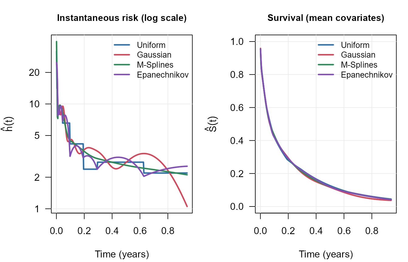
All four bases agree on the broad picture: a hazard that falls steeply over the first few weeks and then levels off, and survival curves that are nearly identical. The hazard estimates themselves are not nearly identical, and the log scale is what shows it. The uniform basis gives the expected step artefacts, while the three smooth bases oscillate, and disagree about where the peaks and troughs fall, because smooth = 0 applies no roughness penalty at all. Penalised fits (smooth > 0, or smooth.per = TRUE for automatic selection) damp these oscillations. That the four disagree this much on $\hat h_0$ while agreeing on $\hat S_0$ is the usual picture: the survival curve integrates the hazard, and integration smooths the differences away.

These are predictions at the mean covariate vector, so each curve estimates $h_0(t)\exp(\bar{\mathbf{x}}^T\boldsymbol{\beta})$ rather than $h_0(t)$ itself. The covariates are not centred, so the level of these curves is not the level of the baseline hazard.

Practical guidance

"msplines" (default for interval-censored data) - M-splines offer a good balance of smoothness and computational efficiency. The second-order roughness penalty has an exact closed form.
"uniform" - fast and simple; useful as a baseline comparison. Use more knots (n.knots) if the hazard is not close to piecewise-constant.
"gaussian" - smooth, kernel-based; both first- and second-order roughness penalties are available. Can be slow with many knots.
"epanechnikov" - compact support like M-splines but with parabolic rather than polynomial shape; only the second-order penalty is supported.

Extensibility

The basis registry (R/basis.R) allows new basis types to be added without modifying existing code. Each basis lives in its own R/basis-*.R file, which implements the three required functions - knots_fn, matrix_fn and penalty_fn - collects them in a spec list, and is registered by a call to register_basis() in zzz.R. Any of the four files is a working template for a fifth basis. See ?list_bases for the bases currently registered.

References

Ma, Jun, Stephane Héritier, and Serigne N. Lo. 2014. “On the Maximum Penalized Likelihood Approach for Proportional Hazard Models with Right Censored Survival Data.” Computational Statistics & Data Analysis 74: 142–56. https://doi.org/10.1016/j.csda.2014.01.005.

Ma, Jun, Annabel Webb, and Harold Malcolm Hudson. 2024. Likelihood Methods in Survival Analysis: With R Examples. 1st ed. Chapman; Hall/CRC. https://doi.org/10.1201/9781351109710.