Comparing coxph() and coxph_mpl() • survivalMPL

Overview

survival::coxph() maximises the partial likelihood - a function of regression coefficients $\boldsymbol{\beta}$ only, with the baseline hazard $h_0(t)$ profiled out. survivalMPL::coxph_mpl() maximises the penalised full likelihood, estimating $\boldsymbol{\beta}$ and $h_0(t)$ jointly via a smooth basis expansion.

For right-censored data with non-informative censoring the two approaches produce essentially the same $\hat{\boldsymbol{\beta}}$ and standard errors (Ma et al. 2014), while coxph_mpl additionally delivers a smooth, closed-form $\hat{h}_0(t)$ that can be plotted and predicted without additional post-processing.

This tutorial uses the lung dataset (survival package) - 228 patients with advanced lung cancer, right-censored overall survival to compare:

Regression coefficient estimates and standard errors.
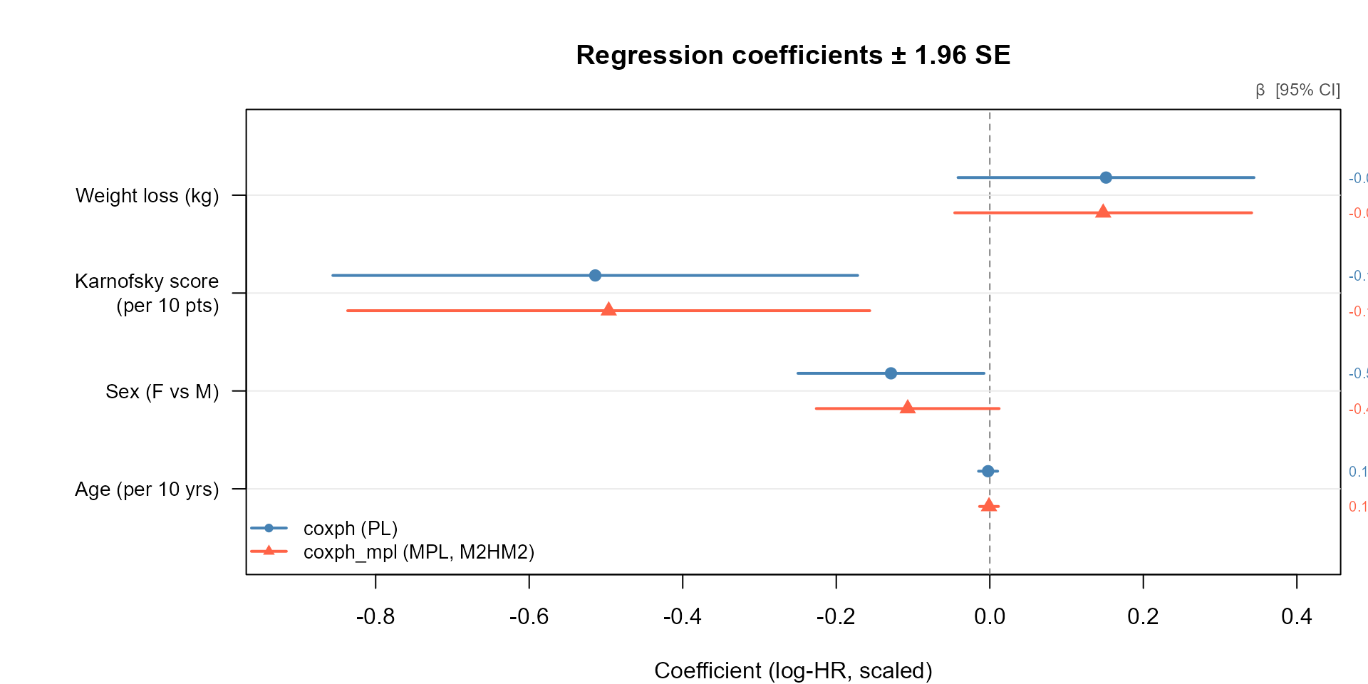
95 % confidence intervals (forest plot).
Estimated baseline survival: Kaplan-Meier, Breslow (from coxph), and M-spline (from coxph_mpl).

Data and model fits

library(survivalMPL)
#> Loading required package: survival
#> Loading required package: MASS
library(survival)

lung <- na.omit(lung[, c("time", "status", "age", "sex", "ph.karno", "wt.loss")])
f    <- Surv(time, status == 2) ~ age + sex + ph.karno + wt.loss

# --- partial likelihood (coxph) ---
fit_pl <- coxph(f, data = lung, x = TRUE)

# --- penalised full likelihood, M-splines (coxph_mpl) ---
fit_mpl <- coxph_mpl(f, data = lung,
  control = coxph_mpl.control(
    basis    = "msplines",
    n.obs    = sum(lung$status == 2),
    max.iter = c(150, 7.5e4, 1e6)
  )
)

Regression coefficients and standard errors

beta_pl  <- coef(fit_pl)
se_pl    <- sqrt(diag(vcov(fit_pl)))

beta_mpl <- coef(fit_mpl)
se_mpl   <- fit_mpl$se$Beta$M2HM2

row_labels <- c(
  age      = "Age (per year)^a^",
  sex      = "Sex",
  ph.karno = "Karnofsky score (per point)^a^",
  wt.loss  = "Weight loss (kg)"
)

tab <- data.frame(
  Covariate    = row_labels[names(beta_pl)],
  `PL est.`    = round(beta_pl,  4),
  `PL SE`      = round(se_pl,    4),
  `MPL est.`   = round(beta_mpl, 4),
  `MPL SE`     = round(se_mpl,   4),
  `Difference` = round(beta_mpl - beta_pl, 4),
  check.names  = FALSE,
  row.names    = NULL
)
knitr::kable(tab, align = "lrrrrr",
             caption = "^a^ The forest plot rescales these covariates to per-10-unit changes.")

^a The forest plot rescales these covariates to per-10-unit changes.
Covariate	PL est.	PL SE	MPL est.	MPL SE	Difference
Age (per year)^a	0.0151	0.0098	0.0148	0.0099	-0.0004
Sex	-0.5140	0.1744	-0.4964	0.1735	0.0176
Karnofsky score (per point)^a	-0.0129	0.0062	-0.0107	0.0061	0.0022
Weight loss (kg)	-0.0022	0.0064	-0.0010	0.0063	0.0012

The estimates agree closely: the full-likelihood approach recovers the same regression signal as partial likelihood, with near-identical standard errors. The MPL SE reported here uses the sandwich variance estimator for a fixed smoothing parameter derived in Ma et al. (2014) (equation 29), accessed via se = "M2HM2" in the package.

Forest plot

Baseline survival comparison

Three survival estimators are overlaid:

Kaplan-Meier - nonparametric marginal estimate, no covariate adjustment. Serves as a visual reference for the raw data.
Breslow - step-function baseline from coxph evaluated at mean covariates via survfit(). This is the standard Cox output for $\hat{S}(t \mid \bar{\mathbf{x}})$ .
M-splines (MPL) - smooth closed-form estimate from coxph_mpl, also evaluated at mean covariates.

Breslow and M-splines estimate the same quantity $\hat{S}(t \mid \bar{\mathbf{x}})$ and should track each other closely. Kaplan-Meier sits apart because it does not adjust for covariates.

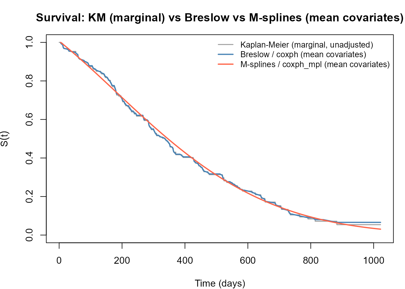
The Breslow estimate is a step function that jumps only at observed event times. The M-spline estimate is smooth by construction and closely tracks the Breslow curve, while avoiding the staircase artefacts that arise from tied or sparse event times. The Kaplan-Meier curve sits above both because it is not adjusted for covariates - in particular it does not account for the protective effect of female sex and higher Karnofsky score at the mean covariate profile.

Instantaneous hazard comparison

Survival curves are the forgiving comparison: integration smooths away differences in the hazard. The instantaneous hazard $\hat h(t)$ is where the two approaches genuinely differ, and it is the quantity coxph() does not estimate at all.

The partial likelihood gives a cumulative hazard that jumps at each event time, so its “hazard” is a set of point masses. To draw it as a rate it has to be binned: the increments of the Breslow cumulative hazard are accumulated over equal-width intervals and divided by the interval width, which is the piecewise-constant hazard estimate implied by coxph() at that resolution. coxph_mpl() needs no such post-processing - $\hat h(t)$ is part of the fitted object.

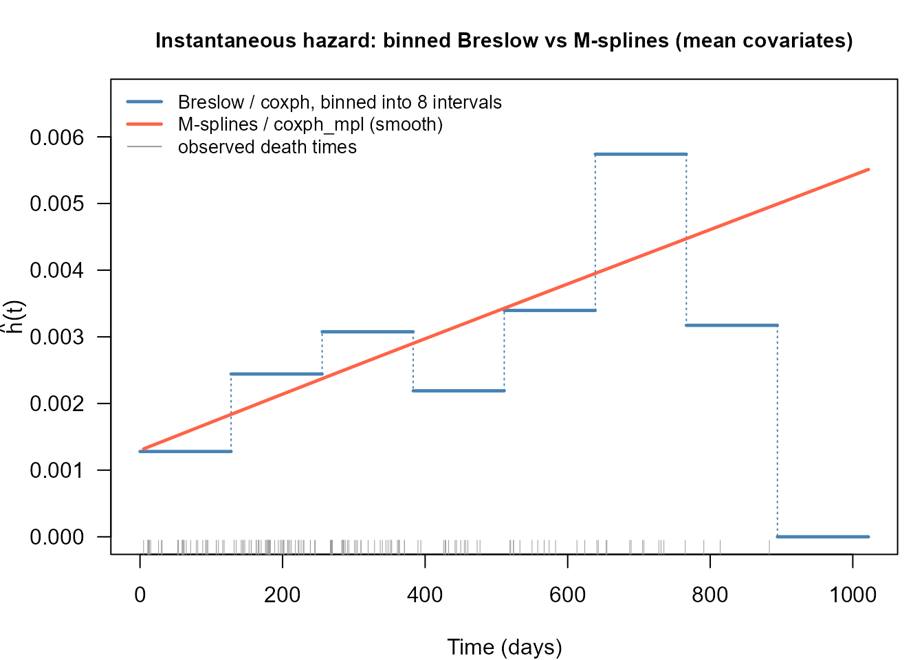
Over the bulk of follow-up the two agree: a hazard of roughly $1.3 \times 10^{-3}$ per day early on, rising to around $3 \times 10^{-3}$ by day 500. The disagreement is in the character of the two estimates rather than their level.

The binned Breslow estimate jumps from bin to bin - its fourth bin sits below its third - and the whole picture depends on a bin width nobody chose on statistical grounds: eight bins give this, sixteen would give something visibly rougher, four something visibly flatter. Its last bin is exactly zero, because no death is recorded after day 894, which is a statement about this sample rather than about the hazard. The M-spline estimate is smooth by construction, with the roughness penalty rather than an arbitrary bin width deciding how much structure survives, and every point of it carries a standard error - which the binned version does not.

Past about 900 days the two part company completely: the smooth estimate goes on rising while the binned one collapses to zero. Neither is informative there. Three patients are still at risk and none of them dies, so the data contain almost nothing about the hazard at that point, and each method fills the vacuum in its own way - one by extrapolating its trend, the other by reporting the empty bin as a zero rate.

That difference is the practical argument for the penalised full likelihood: when the target is a hazard ratio, coxph() and coxph_mpl() agree, and the partial likelihood is the cheaper route; when the target is absolute risk - a hazard, a survival probability, a predicted event time for a given covariate profile - the baseline has to be estimated, and coxph_mpl() estimates it as part of the model.

References

Ma, Jun, Stephane Héritier, and Serigne N. Lo. 2014. “On the Maximum Penalized Likelihood Approach for Proportional Hazard Models with Right Censored Survival Data.” Computational Statistics & Data Analysis 74: 142–56. https://doi.org/10.1016/j.csda.2014.01.005.