Control Parameters

Overview

coxph_mpl() runs with defaults that work for most datasets, so the tutorials call it with nothing but a formula and a data frame. When a fit needs tuning - a different baseline hazard basis, more or fewer knots, a fixed smoothing value, longer iteration limits - the settings live in coxph_mpl.control().

There are two equivalent ways to change them:

# 1. pass control arguments directly; coxph_mpl() forwards them
coxph_mpl(Surv(time, status) ~ x, data = df, basis = "msplines", tol = 1e-5)

# 2. build the control object explicitly
coxph_mpl(Surv(time, status) ~ x, data = df,
          control = coxph_mpl.control(n.obs = sum(df$status),
                                      basis = "msplines", tol = 1e-5))

The first form is shorter and is what the other articles use. The second is needed when the same settings are reused across several fits. Note the n.obs argument in the second form: coxph_mpl.control() uses the number of fully observed events to set defaults, and cannot count them itself, so a hand-built control object must be told. Called through ..., coxph_mpl() counts them for you.

A control object is a plain list with validated entries:

library(survivalMPL)
#> Loading required package: survival
#> Loading required package: MASS
library(survival)

str(coxph_mpl.control(n.obs = 165))
#> List of 16
#>  $ basis            : chr "uniform"
#>  $ smooth           : num 0
#>  $ max.iter         : int [1:3] 150 75000 1000000
#>  $ tol              : num 1e-07
#>  $ order            : int 3
#>  $ penalty          : int 2
#>  $ n.knots          : num [1:2] 8 2
#>  $ range.quant      : num [1:2] 0.075 0.9
#>  $ cover.sigma.quant: num 0.25
#>  $ cover.sigma.fixed: num 0.25
#>  $ n.events_basis   : int 10
#>  $ min.theta        : num 1e-10
#>  $ ties             : chr "epsilon"
#>  $ seed             : int(0) 
#>  $ kappa            : num 1.67
#>  $ epsilon          : num [1:2] 1e-16 1e-10
#>  - attr(*, "class")= chr "coxph_mpl.control"

Every argument is validated on the way in: values outside their admissible range are silently replaced by the default rather than passed on to the optimiser, so an impossible setting cannot produce a meaningless fit.

The baseline hazard

`basis`

Which family of non-negative functions $\psi_1,\ldots,\psi_m$ is used to build $h_0(t) = \sum_u \theta_u \psi_u(t)$ :

Value	Aliases	Shape
`"uniform"`	`"u"`, `"uni"`	Piecewise-constant step functions (default)
`"msplines"`	`"m"`, `"ms"`	M-splines of order `order`
`"gaussian"`	`"g"`, `"gauss"`	Truncated Gaussian kernels
`"epanechikov"`	`"e"`, `"epa"`, `"epanechnikov"`	Epanechnikov kernels

"uniform" is the fastest and gives coefficients $\theta_u$ that read directly as the hazard rate on knot interval $u$ . "msplines" is the usual choice when a smooth $\hat h_0$ matters, in particular for interval-censored data where $H_0$ enters the likelihood at both endpoints. Basis Functions for the Baseline Hazard defines each one and compares them on the same data.

`n.knots` and `range.quant`

n.knots is a length-2 vector c(k1, k2). The first entry places $k_1 + 1$ knots at quantiles of the observed event times up to range.quant[2] (the 90th percentile by default); the second places $k_2 + 1$ equally spaced knots above that quantile. When k2 = 0, all knots are quantile-based over the whole range. Defaults are c(8, 2) for "uniform" and "msplines", and c(0, 20) for the two kernel bases.

More knots mean a more flexible $\hat h_0$ and a larger $\boldsymbol{\theta}$ to estimate; the penalty, not the knot count, is what should control smoothness, so a moderately generous knot count with automatic smoothing is usually better than a small one:

lung <- na.omit(lung[, c("time", "status", "age", "sex", "ph.karno", "wt.loss")])
f    <- Surv(time, status == 2) ~ age + sex + ph.karno + wt.loss

fit_coarse <- coxph_mpl(f, data = lung, n.knots = c(3, 1),  tol = 1e-5)
fit_fine   <- coxph_mpl(f, data = lung, n.knots = c(15, 3), tol = 1e-5)

c(coarse = fit_coarse$knots$m, fine = fit_fine$knots$m)
#> coarse   fine 
#>      5     19
round(cbind(coarse = coef(fit_coarse), fine = coef(fit_fine)), 4)
#>           coarse    fine
#> age       0.0145  0.0142
#> sex      -0.5077 -0.5087
#> ph.karno -0.0116 -0.0119
#> wt.loss  -0.0016 -0.0018

The regression coefficients barely move; what changes is the resolution of the baseline hazard.

par(mfrow = c(1, 2), mar = c(4, 4, 3, 1))
plot(fit_coarse, which = 2, ask = FALSE, cex.main = 0.85)
plot(fit_fine,   which = 2, ask = FALSE, cex.main = 0.85)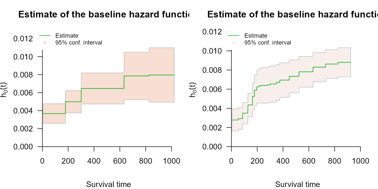

`order` and `penalty`

order is the order of the M-spline or Epanechnikov basis (default 3, cubic M-splines). Order 1 M-splines coincide with the uniform basis and order 2 with a triangular basis.

penalty is the order of the roughness penalty: 1 penalises the first differences of $\boldsymbol{\theta}$ , 2 the second differences. The uniform and Gaussian bases accept either; the Epanechnikov basis always uses second order, and M-splines use order - 1. The default is 2.

Smoothing: `smooth`

The penalised log-likelihood maximised by coxph_mpl() is

$\Phi(\boldsymbol{\beta},\boldsymbol{\theta}) = \ell(\boldsymbol{\beta},\boldsymbol{\theta}) - \lambda\,\boldsymbol{\theta}^T \mathbf{R} \boldsymbol{\theta},$

where $\mathbf{R}$ is the roughness matrix of the chosen basis and $\lambda \ge 0$ is the smoothing value (Ma et al. 2014). smooth sets $\lambda$ :

`smooth`	Effect
`NULL` (default)	$\lambda$ selected automatically from the data
`0`	No penalty at all: plain maximum likelihood
any $\lambda > 0$	$\lambda$ held fixed at that value

Automatic selection is the default, and is the marginal likelihood method of Ma et al. (2024) (Section 2.10). The quadratic penalty $\boldsymbol{\theta}^T\mathbf{R}\boldsymbol{\theta}$ is read as a normal prior $\boldsymbol{\theta} \sim N(\mathbf{0}, \sigma^2\mathbf{R}^{-1})$ with $\sigma^2 = 1/(2\lambda)$ ; $\boldsymbol\beta$ and $\boldsymbol\theta$ are integrated out, and a Laplace approximation to the resulting marginal likelihood gives the update $\hat\sigma^2 = \hat{\boldsymbol\theta}^T\mathbf{R}\hat{\boldsymbol\theta}/\nu$ , where $\nu$ is the model degrees of freedom. Since the estimates and $\sigma^2$ depend on each other, this alternates: inner iterations fit $\boldsymbol\beta$ and $\boldsymbol\theta$ at the current $\sigma^2$ , then an outer iteration updates $\sigma^2$ , until $\nu$ stabilises.

Whether $\lambda$ was selected or fixed is visible in the fitted object: supplying smooth sets max.iter[1] to 1, which switches the outer iterations off, and summary() reports the value as fixed rather than estimated. The final $\lambda$ - selected or not - is stored in fit$control$smooth.

fit_ml   <- coxph_mpl(f, data = lung, smooth = 0)      # unpenalised
fit_auto <- coxph_mpl(f, data = lung)                  # automatic smoothing value
fit_hard <- coxph_mpl(f, data = lung, smooth = 1e8)    # heavily penalised

c(ml = fit_ml$control$smooth,
  automatic = fit_auto$control$smooth,
  hard = fit_hard$control$smooth)
#>        ml automatic      hard 
#>         0  19163433 100000000

Choosing $\lambda$ by hand

$\lambda$ is not scale-free. It trades off against the size of $\boldsymbol{\theta}$ , which depends on the time units, the basis and the number of knots, so the value that oversmooths one dataset is negligible on another - the selected value above is of order $10^7$ only because lung measures time in days, making the hazard rates themselves of order $10^{-3}$ . There is no portable rule of thumb, which is the reason to leave smooth = NULL unless there is a specific reason not to. If a fixed value is needed, fit a small grid and inspect $\hat h_0$ , rather than transplanting a value from another analysis. Extremely large values eventually break the fit rather than flattening it: on lung, $\lambda = 10^9$ drives the estimate to a degenerate solution with an attenuated sex coefficient.

The optimiser

Argument	Meaning	Default
`max.iter`	Length-3 vector: (1) outer smoothing-parameter updates, (2) inner $\boldsymbol\beta$ / $\boldsymbol\theta$ updates, (3) total inner iterations	`c(150, 7.5e4, 1e6)`
`tol`	Convergence tolerance: on the parameter change between inner iterations, and, as `10 * tol`, on the change in the degrees of freedom $\nu$ between outer iterations	`1e-7`
`kappa`	Step-size reduction factor (> 1) applied when the penalised likelihood fails to increase	`1/0.6`
`min.theta`	$\hat\theta_u$ below this are reported as zero, i.e. as active non-negativity constraints	`1e-10`
`epsilon`	Length-2 floor on survival and baseline hazard values, guarding the logarithms	`c(1e-16, 1e-10)`

Setting smooth to a fixed value forces max.iter[1] to 1, since there is no outer loop left to run. summary() prints whether the algorithm converged and how many outer and inner iterations it used; fit$iter holds the same two numbers:

fit_auto$iter        # c(outer iterations, total inner iterations)
#> [1]  150 4268

If either equals its cap the fit has not converged, and summary() says Convergence: NO. fit_auto above is such a fit: with everything at its default it stops at the cap of 150 outer iterations without the degrees of freedom having settled.

The reason is the stopping rule rather than the data. The outer loop stops when $\nu$ changes by less than 10 * tol, which is $10^{-6}$ at the default tol = 1e-7, whereas Ma et al. (2024) describe stability in $\nu$ as changes “not greater than, say, 1 or 0.5”. Asking for six decimal places of a quantity the method itself treats as settled at half a unit is what keeps the loop running. Either loosening tol to the $10^{-5}$ the book uses in its own examples, or raising the cap, produces the same fit:

fit_tol  <- coxph_mpl(f, data = lung, tol = 1e-05)
fit_more <- coxph_mpl(f, data = lung, max.iter = c(600, 7.5e4, 1e6))

rbind(`tol = 1e-05`  = fit_tol$iter,
      `max.iter 600` = fit_more$iter)
#>              [,1] [,2]
#> tol = 1e-05   101  571
#> max.iter 600  492 5196

round(cbind(`default (capped)` = coef(fit_auto),
            `tol = 1e-05`      = coef(fit_tol),
            `max.iter 600`     = coef(fit_more)), 4)
#>          default (capped) tol = 1e-05 max.iter 600
#> age                0.0146      0.0144       0.0146
#> sex               -0.5108     -0.5103      -0.5108
#> ph.karno          -0.0118     -0.0117      -0.0118
#> wt.loss           -0.0018     -0.0017      -0.0018

The three sets of coefficients differ by at most a twentieth of a standard error, so the capped fit was not wrong - but a fit that reports non-convergence should not be published on the strength of that, and tol = 1e-05 is the cheaper of the two ways out. If neither helps, the usual causes are too many knots for the number of events, or a covariate on a very different scale from the others.

Ties: `ties` and `seed`

Knot sequences are built from the distinct fully observed event times. Duplicated event times therefore have to be resolved:

ties = "epsilon" (default) jitters duplicates by a small random amount;
ties = "unique" drops duplicates before computing quantiles.

Because "epsilon" uses the random number generator, seed fixes it so the knots - and hence the fit - are exactly reproducible:

fit_a <- coxph_mpl(f, data = lung, ties = "epsilon", seed = 42)
fit_b <- coxph_mpl(f, data = lung, ties = "epsilon", seed = 42)
identical(coef(fit_a), coef(fit_b))
#> [1] TRUE

The current RNG state is restored afterwards, so setting seed does not disturb any simulation running around the fit.

Full argument list

Argument	Purpose
`n.obs`	Number of fully observed events; used to derive defaults
`basis`	Basis for $h_0$
`smooth`	Smoothing value $\lambda$ ; `NULL` = automatic selection, `0` = no penalty
`max.iter`	Iteration limits for the three optimisation stages
`tol`	Convergence tolerance
`n.knots`	Quantile and equally spaced internal knot counts
`range.quant`	Quantile range for the quantile-based knots
`order`	Order of the M-spline / Epanechnikov basis
`penalty`	Order of the roughness penalty
`cover.sigma.quant`, `cover.sigma.fixed`	Bandwidth targets for the Gaussian basis
`min.theta`	Threshold below which $\hat\theta_u$ is reported as zero
`kappa`	Step-size reduction factor
`epsilon`	Numerical floors for survival and hazard values
`ties`	Tie-breaking strategy for duplicated event times
`seed`	RNG seed used when `ties = "epsilon"`
`n.events_basis`	Events per uniform basis element; retained for backward compatibility, not used by the current knot construction

See ?coxph_mpl.control for the full argument documentation.

Practical recipes

Start with the defaults. Uniform basis, automatic smoothing, default knots.
Interval- or left-censored data: basis = "msplines", since $H_0$ is evaluated at both interval endpoints and a step function makes that estimate coarse.
Comparing bases or reproducing a maximum likelihood fit: smooth = 0.
Left truncation (entry): basis = "uniform" - the only basis for which differencing the cumulative basis is implemented. Any other basis is replaced by "uniform" with a warning.
A fit that will not converge: set tol = 1e-05 first - the outer loop stopping rule at the default tolerance is stricter than the method needs - then raise max.iter, then reduce n.knots.

References

Ma, Jun, Stephane Héritier, and Serigne N. Lo. 2014. “On the Maximum Penalized Likelihood Approach for Proportional Hazard Models with Right Censored Survival Data.” Computational Statistics & Data Analysis 74: 142–56. https://doi.org/10.1016/j.csda.2014.01.005.

Ma, Jun, Annabel Webb, and Harold Malcolm Hudson. 2024. Likelihood Methods in Survival Analysis: With R Examples. 1st ed. Chapman; Hall/CRC. https://doi.org/10.1201/9781351109710.

Overview

The baseline hazard

basis

n.knots and range.quant

order and penalty

Smoothing: smooth

Choosing λ\lambda by hand